Galileo flow rate sensor comparative performance
Author
Lisa Muiznieks, PhD
Publication Date
Keywords
flow measurement
sensor performance
flow sensor
comparative analysis
flow accuracy
flow control
Need advice for chosing your flow sensor?
Your microfluidic SME partner for Horizon Europe
We take care of microfluidic engineering, work on valorization and optimize the proposal with you
Introduction
Microfluidics is a powerful tool to add perfusion to a diverse range of experiments on the microscale. In the biology field, perfusion can turn a static cell culture chamber into a microenvironment with flow to mimic physiological conditions. For example, flow can be modulated to represent vascular flows, interstitial flow or lymphatic drainage.
Applications of adding flow to cell assays are wide and varied such as cell rolling-adhesion, tumor metastasis, molecular transport, metabolism and microphysiological systems (MPS or organ-on-chip). Practical advantages of perfusion include nutrients exchange, medium conditioning, waste removal, and the addition of shear stress as a mechanical stimulus.
Flow setups further enable the automated addition of reagents, collection of samples in real-time for dynamics studies, or the continuous sensing of parameters.
The backbone of a perfusion setup is the pump to move the liquid. A flow rate sensor is a key component that can provide highly complementary flow rate measurement and/or control to perfusion setups. In particular, an inline flow sensor will allow you to measure the flow profile of your pumping system, including measuring the stability and pulsatility of your flow profile or accuracy of your pump.
Our new Galileo flow rate sensor is compatible for use with any pump, including pressure-based pumps, syringe pumps and peristaltic pumps.
The Galileo flow rate sensor is designed with a base and snap-in cartridge format. The flow path is contained entirely within the cartridge that can be swapped to measure different flow rate ranges, or when it is important to avoid cross-contamination between experiments. Our sensor also features a unique clogging alert light to notify the user that the measurement reading is drifting or if the sensor is fully blocked.
This application note compares the performance of our Galileo flow rate sensor to two of the most commonly available flow sensors on the market today, Bronkhorst and Sensirion flow sensors. We use a pressure controller pump for maximum flow stability.
Applications
Applications of the Galileo flow rate sensor in microfluidic cell culture experiments and cell assays are diverse. The following examples are not exhaustive:
- Cell culture under flow
- Microfluidic cell assays (e.g. cell attachment, migration, metastasis)
- Microphysiological systems (MPS, organ-on-chip)
- Molecular transport (e.g. drug toxicity, absorption, filtration, blood-brain-barrier)
- Droplet microfluidics (e.g. cell encapsulation, double emulsions, nanoparticle formation)
- Measure the pulsatility of your flow profile to assess how it affects your cells
- Monitor the accuracy and stability of your pump
Setup
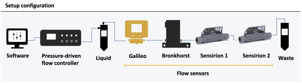
In this setup, a pressure-driven flow controller (OB1 MK4, Elveflow) was used to push the liquid. The Galileo flow rate sensor was connected inline before a Bronkhorst mini CORI-FLOW digital mass flow meter and two Sensirion flow sensors, LG16-0431D (Sensirion 1) and LG16-1000D (Sensirion 2).
Materials
Hardware:
- Flow controller (e.g. pressure-driven OB1 MK4 with one 0-2000 mbar channel, Elveflow)
- Galileo flow rate sensor (6-200 µl/min cartridge used here; Note: other ranges are available)
- Comparison flow sensors, Bronkhorst (1.6 µl/min – 3 ml/min; 0.2% accuracy) and Sensirion (2-80 µl/min, range of 5% accuracy, Sensirion 1; and 40-1000 µl/min, range of 5% accuracy, Sensirion 2)
- Tubings (PTFE, 1/16” outer diameter; OD), fittings and reservoirs
Chemicals:
- Distilled water, filtered
Quick start guide
Instrument connection
1. Connect your OB1 pressure controller to an external pressure supply using pneumatic tubing, and to a computer using a USB cable. For detailed instructions on OB1 pressure controller setup, please read the “OB1 User Guide”.
2. Turn on the OB1 by pressing the power switch.
4. Press Add instrument \ choose OB1 \ set as MK4, set pressure channels if needed, give a name to the instrument and press OK to save changes. Your OB1 should now be on the list of recognized devices.
7. Connect the Galileo flow rate sensor base to your computer with a USB cable.
8. Insert the flow sensor cartridge into the base.
9. Open the Galileo software. (Download the software)
11. OPTIONAL: Connect additional flow rate sensors to the OB1 MK4.
Note: This application note compares the performance of the Galileo flow sensor to other commercially available flow sensors. One flow sensor is normally sufficient for a regular experiment.
Setup preparation
1. Connect the reservoir caps to the OB1 with pneumatic tubing.
2. Connect the reservoir to the Galileo flow sensor cartridge inlet with 1/16” OD tubing.
3. OPTIONAL: Connect a Bronkhorst flow sensor followed by Sensirion flow sensors spanning the desired flow measurement range using 1/16” OD tubing. Here we used a Bronkhorst mini CORI-FLOW digital mass flow meter and Sensirion LG16-0431D and LG16-1000D flow sensors.
Pressure profile configuration
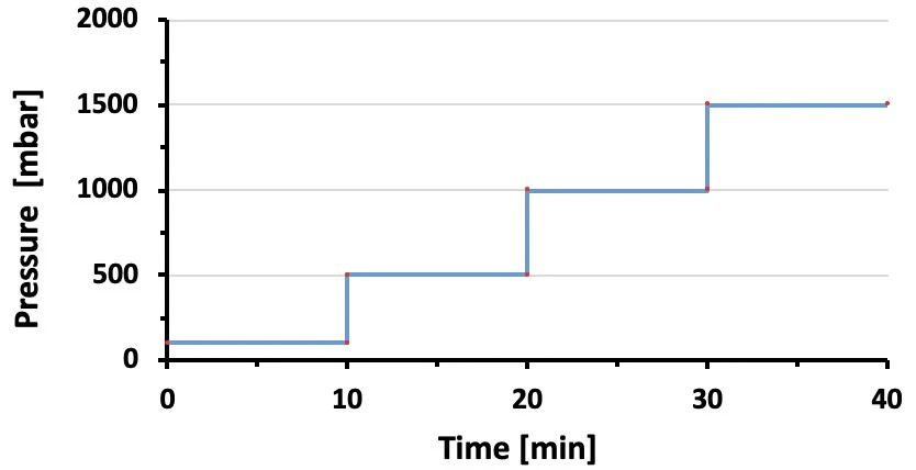
1. Prepare a pressure step profile spanning the measurement range of the flow sensor of interest using the ESI (Elveflow software used to control the OB1; Fig. 1).
Experiment
1. Start Galileo acquisition on the software interface (acquisition sampling time 0.1 s)
2. Start the pressure sequence.
Download the MIC Horizon Europe 2026/2027 Calls Calendar:
Results
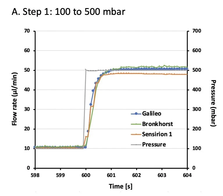
A series of pressure steps were set spanning a flow range from ~10 – 150 µl/min. Galileo and Sensirion flow rate sensor data were compared to Bronkhorst flow sensor values at each pressure step (Figures 2, 3).
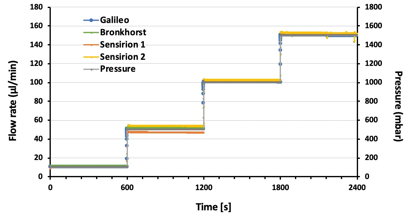
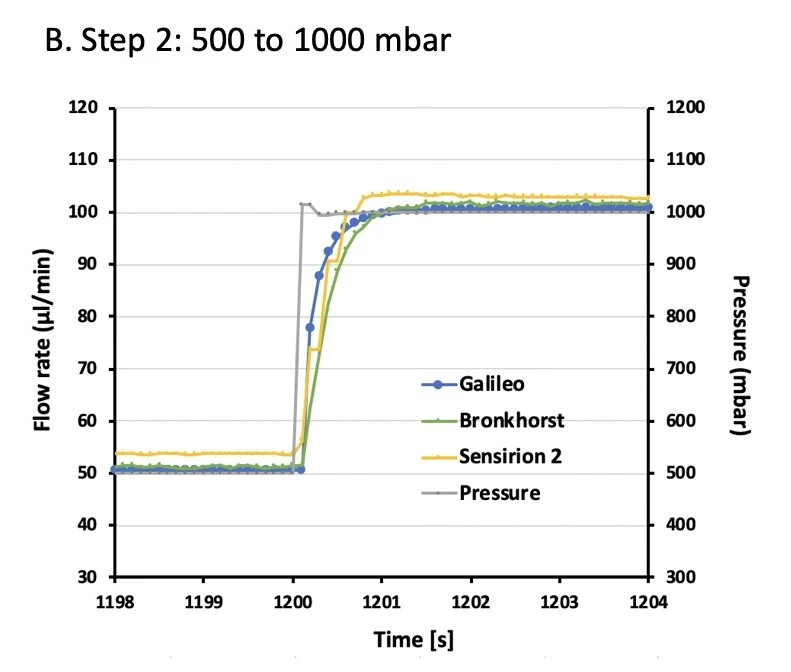
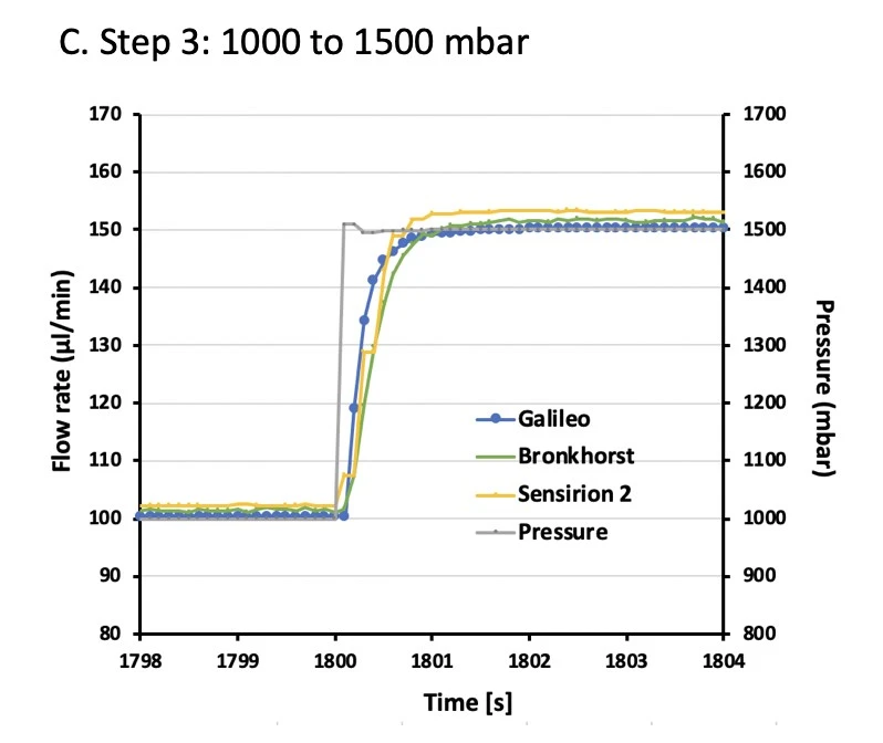
Data were analyzed for accuracy and stability. Accuracy was calculated for each pressure step as the average of 500 s of data (i.e. between 50-550 s of each step). Error is shown as the percent deviation compared to the Bronkhorst flow sensor (Table 1).
Table 1. Accuracy of the Galileo flow rate sensor as a percent error relative to a Bronkhorst flow sensor (reference). Measured Sensirion flow sensor accuracy is also given. Galileo was within 5% accuracy across the whole flow rate range tested (n=3).
| Pressure step: 100 mbar | ||||
| Sensor name | Galileo | Bronkhorst | Sensirion 1 | Sensirion2 |
| Average error % | 3.159 | reference | 4.604 | out of range |
| Pressure step: 500 mbar | ||||
| Sensor name | Galileo | Bronkhorst | Sensirion 1 | Sensirion 2 |
| Average error % | 1.678 | reference | 8.958 | 4.700 |
| Pressure step: 1000 mbar | ||||
| Sensor name | Galileo | Bronkhorst | Sensirion 1 | Sensirion 2 |
| Average error % | 0.799 | reference | out of range | 0.597 |
| Pressure step: 1500 mbar | ||||
| Sensor name | Galileo | Bronkhorst | Sensirion 1 | Sensirion 2 |
| Average error % | 0.593 | reference | out of range | 0.774 |
Stability was calculated as the sample variance (spread) over 100 s of data for each pressure step (i.e. from 400-500 s of each step; Table 2).
Table 2. Average stability of the Galileo flow rate sensor at each pressure step. Measured Bronkhorst and Sensirion flow sensor stability is also given (n=3). Galileo displayed a sample variance of 1-3 orders of magnitude smaller than the other flow sensors.
| Pressure step: 100 mbar | ||||
| Sensor name | Galileo | Bronkhorst | Sensirion 1 | Sensirion2 |
| Average variance | 0.000052 | 0.055690 | 0.000470 | out of range |
| Pressure step: 500 mbar | ||||
| Sensor name | Galileo | Bronkhorst | Sensirion 1 | Sensirion 2 |
| Average variance | 0.000059 | 0.063217 | 0.004844 | 0.010891 |
| Pressure step: 1000 mbar | ||||
| Sensor name | Galileo | Bronkhorst | Sensirion 1 | Sensirion 2 |
| Average variance | 0.00032 | 0.06292 | out of range | 0.01343 |
| Pressure step: 1500 mbar | ||||
| Sensor name | Galileo | Bronkhorst | Sensirion 1 | Sensirion 2 |
| Average variance | 0.0029 | 0.1370 | out of range | 0.1130 |
More tips included in the Application Note PDF!

Acknowledgements
This application note is part of a project that has received funding from the European Union’s Horizon research and innovation program under HORIZON-EIC-2022-TRANSITION-01, grant agreement no. 101113098 (GALILEO).
This application note was written by Lisa Muiznieks, PhD.
Published on June 2024
Contact: Partnership[at]microfluidic.fr

Check the other Application Notes
FAQ - Galileo flow rate sensor comparative performance
How does one interpret what this note contrasts?
This page compares the performance of the inline Galileo sensor with that of conventional flow sensors – specifically, the setpoint of a syringe pump, weight-based collection over time, and inferred flow from pressure readings. The pump’s input values appear precise yet theoretical; they reflect intent more than reality. Gravimetric methods reliably capture actual volume changes, though their pace limits their usefulness during fast experiments. Pressure-derived estimates respond quickly but depend heavily on assumptions about system behavior. Meanwhile, Galileo delivers measured flow data directly within the channel, synchronized with ongoing reactions. It avoids delays, gives immediate feedback, and sits exactly where processes unfold. Unlike indirect indicators, it reports what actually occurs, not what should. Speed meets accuracy without stepping outside the device.
What about Galileo’s position regarding low-flow gravimetry?
In the typical 0.5-50 µL/min window used for cell culture, droplet work, and reagent dosing, side-by-side tests generally fall within a few percent of weigh-and-time results once the sensor is matched to the correct cartridge and the fluid is at the experimental temperature. On time-averaged windows (e.g., 60-120 s), the slope of Galileo vs. gravimetry is essentially unity, with high linearity across that range. The practical takeaway is that you can trust the live number for set-and-hold control and keep gravimetry for the occasional audit.
What do we gain over “the syringe pump says 5 µL/min”?
A reading from a pump does not reveal what happens within the fluid path – only what the system intends. What moves through the channel might differ from the set values due to thermal effects, material flexibility, or downstream resistance. One moment it reads five microliters per minute; soon after, it slips to four point four or climbs past five point six. Pulsing flows, slow blockages, or steady deviations remain hidden without direct observation. Measurement at the source misses these shifts entirely. Sensing where the liquid actually travels exposes discrepancies as they arise. Adjustments become possible only when reality is visible.
What speed does the sensor react at when conditions shift?
Faster than a second passes. Flow irregularities – like those from a syringe pump’s pulse, the bumps of peristaltic motion, or shifts when pressure adjusts – show up clearly, no extra filtering needed. Precision here ensures that at minute twelve, each run matches the last, whether delivering doses or timing stimuli.
Can changes in thickness affect measurement accuracy?
Only works when handled carefully. Inside every snap-in unit sits a sensor matched to specific flow rates and tuned to particular thickness levels. Moving from thin liquids to thicker mixtures means replacing these units entirely. Since all contact parts remain sealed, switching prevents mixing of residues. This method maintains accuracy across different fluids.
What happens during extended use – does it resist drifting, manage air pockets, cope with gradual blockages?
Overnight infusions run long – that is when inline monitoring becomes useful. A continuous signal shows slow shifts, even as little as 5 to 10 percent over several hours, missed by setpoint values alone. When a bubble moves through or debris narrows a passage slightly, the change appears instantly in the flow pattern, allowing a response. Built-in visual alerts highlight irregularities or blockages, pulling issues into clear view before they stay buried in small digits.
Could back-pressure or compliance affect results? Might those factors tilt measurements one way?
Flow output shifts when actuators adjust, yet readings stay unbiased. The volume passing through is recorded directly by Galileo. This fits neatly with pressure-based setups: feedback relies on actual flow numbers rather than pressure, since those values drift across devices and over time.
What about Galileo when placed beside differential-pressure or thermal mass sensors under similar conditions?
When working with small fluid volumes and slow flows with water-like liquids, Galileo’s cartridge system sidesteps typical issues. Sensitivity drops due to shifting thickness or reduced warmth; different cartridges handle different ranges. After running samples packed with proteins, leftover gunk rarely sticks around because the liquid is flushed out each time. Heat-based sensors perform well with air or ultra-pure fluids. Pressure-difference techniques work best when flow resistance is known in advance. What sets this apart isn’t flashy – it just works without fuss, connects easily, needs little setup, and holds up when messy biological stuff like blood serum or structural proteins moves through.
How steady will the results be during actual tests? What level of detail can you anticipate?
A steady baseline lasting several hours emerges when the correct cartridge is in place, enabling clear detection of flow shifts as low as one microliter per minute. Mechanical noise fades smoothly with a brief running average – five to ten seconds usually does it – yet actual spikes remain visible. Some data points rise sharply out of the quiet. Researchers often present both unfiltered readings and smoothed curves, along with the smoothing duration. Each lab picks its own span based on system behavior.
Could some constraints catch a reviewer’s attention? What aspects may need clarification ahead of evaluation?
-A single cartridge works best within its specific flow limits; pushing near the edges leaves little margin. What matters is staying centered in that window. Performance drops when the operation skims either end.
-A shift in viscosity or a fluctuation in temperature breaks alignment with calibration settings. When one drifts too far, recalibrate or replace the unit. Precision slips when conditions stray from original specs.
-Bubbles showing up in two separate phases might trick an inline sensor into giving false readings. A small chamber to capture air is best placed right before the microfluidic device. Short lengths of tubing that let gas pass help reduce this issue altogether.
What methods work for checking and recording results when no calibration facility is available?
Do a five-point check against gravimetry at your setpoint band (e.g., 1, 3, 10, 20, 40 µL/min). For each point, collect effluent for a fixed interval (≥10-20 min), convert mass to volume (density near 1.00-1.02 g/mL for most media), and regress Galileo vs. gravimetry. Report slope (~1.00), intercept (near zero), R² (>0.99 desirable), and percent error at each point. Repeat once at operating temperature; viscosity shifts a few percent per °C, which is enough to matter for shear-controlled biology.
How might altering the cartridge setup affect cleanliness and maintenance?
Quite a bit. Since the fluid pathway is sealed inside the cartridge, one can handle sterile or protein-heavy tasks, while the other handles solvents or thick additives. Switching them takes just moments, cuts down leftover volume, limits carryover, and makes quality assurance tracking easier. Every unit acts as its own clear, swappable piece.
How might this appear within a Horizon Europe initiative or during prototype development?
Starting from sensor integration, MIC builds full microfluidic systems centered on devices such as Galileo, incorporating fluid handling, tailored chip shapes, compact tubing layouts, recording tools, and feedback-driven operation. Custom chips are made in-house and shipped as verified models, ready for immediate lab deployment. Because of focused expertise, this small company joins multiple EU collaborative projects, where participation correlates with nearly twice the average approval odds – largely due to method sections shaped by how evaluators assess rigor.
Got a quick tip from personal experience?
Begin by warming the media and removing the gas before calibration. Use a short, rigid upstream line for better stability. Record both the actuator inputs and the actual flow readings. When changing fluid types, replace the cartridge rather than adjusting the zero on the old one. These small steps help maintain consistency between day one and day three.