Microfluidic colocalization set-up for DNA analysis
Author
Lisa Muiznieks, PhD
Publication Date
Keywords
colocalization setup
spatial alignment
imaging
protein detection
sensor integration
DNA analysis
Need advice for your microfluidic colocalization?
Your microfluidic SME partner for Horizon Europe
We take care of microfluidic engineering, work on valorization and optimize the proposal with you
Detect protein and/or DNA interaction with the help of microfluidics
Introduction to microfluidic colocalization
This user guide will show you how to run microfluidic colocalization studies of single-molecule spectroscopy. We will start with the preparation of flow cell and then show you how to apply pressure-driven flow control to liquids for DNA detection studies.
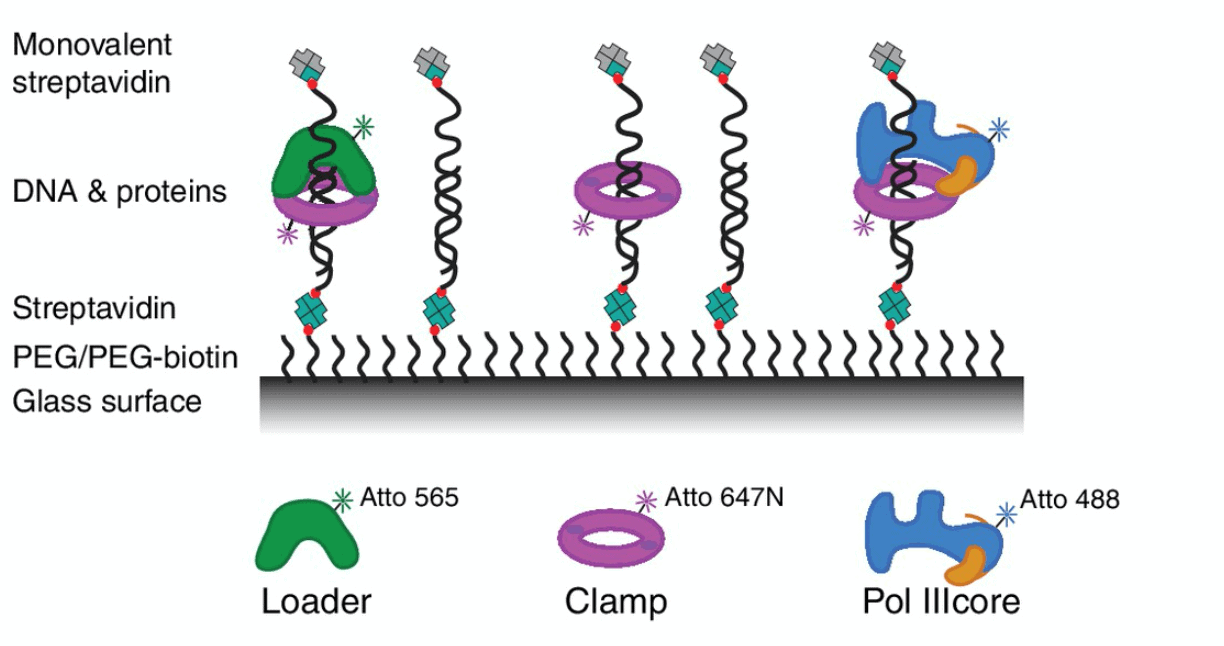
Schematic depiction of DNA and protein colocalization. Single DNA molecules are attached to the glass surface using streptavidin as intermediate bonding agent. In this article we will describe how to perform microfluidic colocalization using an Elveflow setup.
Microfluidic colocalization setup
The imaging chamber consists of a microscope glass slide (1 mm thickness, 25×75 mm size) with etched channels (up to 9 channels on 1 glass slide) covered with a rectangular borosilicate coverslip (0,13 – 0,17 mm thickness, 60 x 22 mm size). The connectors for tubing were bound directly to the microscope glass slide because of its thickness.
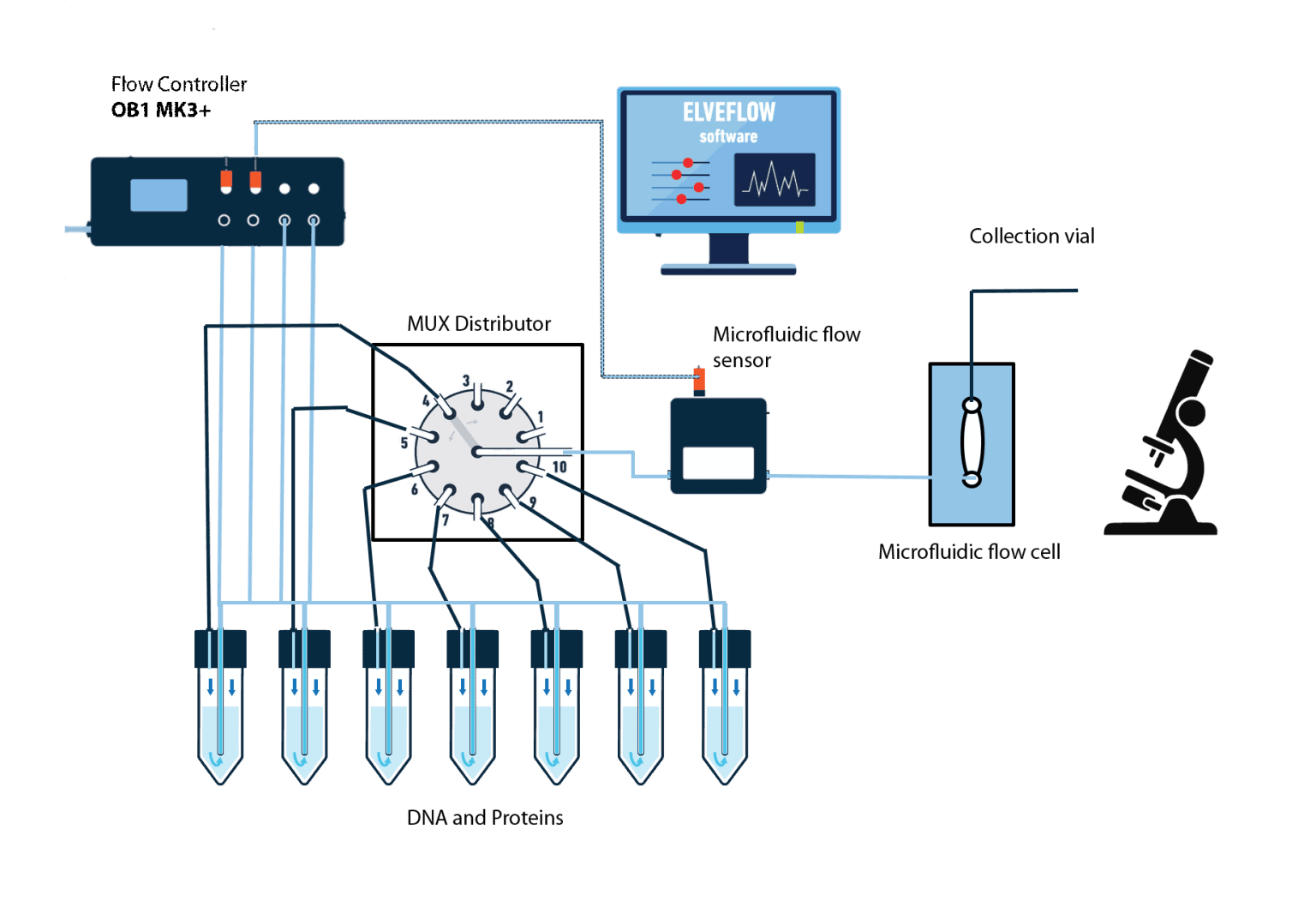
In this experiment, we analyzed several proteins that we introduced into the flow cell using the ELVEFLOW© MUX distribution valve. Using this setup a minimal delay in the sequential injection can be achieved.
Materials for microfluidic colocalization
Hardware:
- OB1 flow controller (Elveflow) with a channel of 0-2000 mbar
- 1 MFS2 flow sensor (Elveflow) 0-7 μL/min
- Kit starter pack luer lock + 1/32 tubings + 1/32 sleeves + custom chip connectors
- 1-8 x 15 mL Falcon reservoirs
- Microfluidic chip
- FRET Microscope for observation
Chemicals:
- 20 mM Tris-HCl pH 7.5
- 50 mM potassium glutamate
- 8 mM MgCl2
- 4% glycerol
- 2 mM DTT
- 0.1% Tween20
- 1 mM Trolox
- Proteins or DNA molecules (Depending on experiment)
Download the MIC Horizon Europe 2026/2027 Calls Calendar:
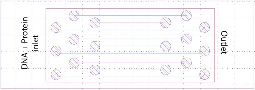
Microfluidic chip design
The bottom part of the chip is made of borosilicate glass, 0.13-0.17 mm. The top glass (cover glass) is a conventional microscope glass slide. The biggest channel length is 40 mm, the smallest 20 mm. Channel depth may differ, here 20-, 30- and 50-micron channels were etched.
The chip was produced by glass etching during the study. Channel width was 150 microns. On the top of the microscope glass slide we drilled inlet and outlet holes. Connectors: custom, made as part of the project. Tubing: external diameter 1 mm.
Quick start guide
Glass surface treatment to preassemble the flow cell
1. Wash the flow cell with bleach and inactivate the bleach with sodium thiosulfate.
2. Flow a solution of neutravidin, then flow with a casein and/or BSA solution to close gaps on the surface.
3. For “sticky” proteins, pre-treatment of the bottom glass slide by means of pre-silanization is usually required.
Bonding of DNA to the glass surface
Tips from the expert
Before starting the experiment, proteins and DNA should be labelled and purified using gel filtration. The extended protocol can be requested (classical protein purification).
4. Connect your OB1 pressure controller to an external pressure supply using pneumatic tubing, and to a computer using the USB cable. For detailed instructions on OB1 pressure-driven flow controller setup, please read the OB1 user guide.
5. Plug the microfluidic reservoir to the OB1 pressure controller outlet. The Elveflow reservoir connection instructions are covered by a specific guide (see Elveflow microfluidic reservoir assembly instructions).
6. For the feedback loop, connect a flow sensor to the OB1. Then, connect flow sensors between the microfluidic reservoirs and the chip for flow measurement.
7. Turn on the OB1 by pressing the power switch.
8. Launch the Elveflow software. The Smart Interface guide covers the Elveflow Smart Interface’s main features and options. Please refer to those guides for a detailed description.
9. Press Add instrument \ choose OB1 \ set as MK4, set pressure channels if required, give a name to the instrument, and press OK to save changes. Your OB1 should now be on the list of recognized devices.
10. OB1 calibration is required for the first use. Please refer to the OB1 user guide.
11. Add flow sensor: press Add sensor \ select flow sensor \ analog or digital \ max flow rate for the sensor, give the sensor a name, select to which device and channel the sensor is connected, and press OK to save the changes. For details refer to the Microfluidic flow sensor user guide.
12. Add MUX distributor: press Add instrument \ choose MUX distribution/injection \ give the instrument a name \ select the number of valves (10 or 12).
13. Connect the OB1 to the manifold and the manifold to all the reservoirs you need.
14. Use the supplied 1/32” OD tubing to connect the microfluidic reservoirs to the MUX distributor and one tubing at the outlet of the MUX distributor. Add a dead-end block to the inlets of the MUX-distributor that are not used.
Tips from the expert
Use consecutive MUX inlets for liquid reservoirs and the dead-end. The MUX will switch liquids following the shortest travel distance. Air will enter the system if the MUX passes over an open inlet.
15. Set pressures (and other parameters if needed) and start pumping liquids into the chip. Wait until all air bubbles escape from the chip and both liquids flow.
Tips from the expert
Chip priming: To begin with, run liquids into tubes until the liquid starts to drip for each inlet of the MUX distribution. Only then, connect them to the chip.
16. Flow continuously at 1µL/min using the flow sensor feedback loop (see Elveflow flow sensor User Guide) the following solutions in this order:
a. 10 µL of PBS
b. 5 µL of bio-BSA 0.1 mg/mL PBS
c. 5 µL of PBS
d. 5 µL of Pluoronics 0.5%
e. 5 µL of Neutravidin 0.2 mg/mL
f. 5 µL of Casein 0.02%
g. 5 µL of 20kb DNA bio (1 µL-0.5 ng) in PCB (19 µL)
Tips from the expert
PBS is phosphate-buffered saline and PCB is PBS with BSA (0.4 mg/mL) and casein (0.02%).
17. Incubate for at least 15 minutes at room temperature without flow.
18. Restart the continuous flow with the following solutions:
a. 5 µL PCB
b. 5 µL Neutravidin 0.2 mg/mL
c. 5 µL of Pluronics 0.5%
Microfluidic setup imaging
19. Different microscope setups can be used, for example, the Nikon (Kingston Upon Thames, United Kingdom) Eclipse Ti-E microscope with the ApoTirf 100X/1.49 Oil, 0.13–0.20 WD 0.12 objective.
20. We used lasers with 150 mW 488 nm, 150 mW 561 nm (both Coherent Sapphire Ely, United Kingdom), and 100 mW 638 nm (Coherent Cube) controlled by an acousto-optic tunable filter (Gooch and Housego, Ilminster, United Kingdom).
21. Each view field is about 50 x 50 microns, channels have a width of 150 microns to observe the molecules in the middle of the channel without any distortion or artifacts.
Congratulations!! You achieved the binding and monitoring of single molecules on chip! We hope this tutorial is a useful guide in your microfluidic experiments. If you need further details or additional information, do not hesitate to contact our experts!
This project has received funding from the European Union’s Horizon 2020 research and innovation programme under the Marie Sklodowska-Curie grant agreement No 722433 (DNARepairMan).
Check the other Application Notes
FAQ - Microfluidic colocalization set-up for DNA analysis
How is the standard configuration arranged?
A single glass slide, measuring 25 x 75 millimeters and roughly 1 millimeter thick, can hold up to 9 carved pathways. These channels are enclosed beneath a thin rectangle of borosilicate cover glass measuring 60 by 22 millimeters, with a thickness of 0.13 to 0.17 millimeters. Holes in the slide serve as entry and exit points, linked directly to a system that regulates fluid flow via pressure. For quick changes between solutions, a switching mechanism directs the incoming streams. Feedback from a flow monitor ensures a consistent liquid supply by enabling real-time adjustments. Visual data collection is performed using a microscope equipped for FRET, epifluorescence, and TIRF imaging.
What kind of equipment do people usually choose – and what drives that choice?
- Pressure controller: OB1 controls the 0-2000 mbar range with high accuracy. Precise, fast transients for clean switching
- Flow sensor: MFS2, 0-7 µL/min, stabilizes to 1 µL/min setpoints.
- Distribution valve: MUX (10-12 ports) – minimal dead volume, low switching delay.
- Reservoirs: 1–8 × 15 mL Falcon-style.
- Chip connectors/tubing: 1/32″ OD lines with custom connectors to the glass slide.
- Microscope: FRET or multi-laser fluorescence.
What drives the structure of a microfluidic chip?
A thin base made of borosilicate glass, between 0.13 and 0.17 millimeters thick, supports the structure above. On top sits a conventional microscope slide. Channels measure approximately 150 micrometers across; their depth may vary between 20, 30, or 50 micrometers, with lengths ranging from 20 to 40 millimeters. Because of this shape, fluid moves smoothly in parallel layers. The viewing area covers roughly 50 by 50 micrometers, centered and positioned away from channel edges to reduce image warping.
Can you outline a fast start-to-finish protocol?
- Surface prep: bleach wash → quench with sodium thiosulfate → coat with neutravidin → block with casein/BSA. For “sticky” proteins, pre-silanize the bottom slide.
- Instrument set-up: connect OB1 to pressure supply and USB; add the flow sensor and MUX in software; calibrate the OB1; define sensors; select MUX size.
- Chip priming: run liquids into tubes until the liquid starts to drip for each inlet of the MUX distribution. Only then, connect them to the chip.
- Flow program at 1µL/min using the flow sensor feedback loop
- Incubate 15 min (no flow), then rinse/condition: 5 µL PCB → 5 µL neutravidin (0.2 mg/mL) → 5 µL Pluronics (0.5%).
- Inject labeled proteins via MUX for colocalization imaging.
What shortcuts prevent delays or frustration?
-Starting from one end, assign sequential MUX ports to reagents while leaving a nearby blind channel. That reduces the distance fluids must travel and prevents the rotor from exposing samples to air during transfer.
-Bubbles cause trouble – prepare each line completely ahead of linking the chip. Before connecting, ensure no air remains inside.
-Start by tagging molecules carefully. Separation by gel filtration removes loose dyes. Impurities, such as clumped proteins, are filtered early. Clean samples prepare the way for accurate readings later.
-A steady flow of 1 microliter per minute helps control the force on the surface during chemical treatment while still allowing full liquid replacement. With this rate, molecules interact gently but thoroughly over time.
Which imaging setup has been tested in real-world conditions for this arrangement?
A setup often includes a Nikon Eclipse Ti-E microscope paired with a 100×/1.49 numerical aperture ApoTIRF oil objective. For illumination, lasers at 25°C deliver light at 488 nm with 150 mW, 561 nm with 150 mW, and 638 nm with 100 mW, controlled via an acousto-optic tunable filter. Positioning the imaging area near the middle of the microfluidic paths, about 150 micrometers wide, ensures observations are roughly 50 by 50 micrometers from the physical boundaries, reducing interference. Camera settings, along with exposure duration shift, are based on dye characteristics and how they interact with light; compounds like Trolox reduce intermittent signal loss during recording.
What speed allows reagent changes without contaminating the mix?
A single pressure regulator paired with a multiplexer allows rapid switching during repeated sample delivery – only the fluid path size holds things back. Moving from one port to the next on the MUX, cutting tube length short, and filling lines ahead of time: these cut inactive periods down to just a few seconds when distances are short. When flow runs at one microliter per minute across channels holding roughly 10 to 20 microliters, stabilization takes about half a minute or more. Pushing the speed up shrinks that interval, though stronger forces act on the liquid in return.
What are common failure modes, and how do I troubleshoot them?
- A weak signal might stem from ineffective DNA attachment. Begin by verifying the biotinylation process worked correctly. Check whether neutravidin remains active – older reagents lose potency. Follow the passivation steps precisely, as sequence matters greatly here. When needed, go beyond the standard 15-minute wait to boost binding. Each stage hinges on careful timing and fresh components.
- Background glow too high? Try stronger blocking – use casein or BSA. Check whether Pluronics were applied properly during washing. Make sure the unbound dye is washed away after labeling.
- Start by removing bubbles through line re-priming. Buffers benefit from degassing before use. A small increase in pressure when changing conditions helps prevent bubble buildup. Finish with a stable flow to maintain clarity.
- Unstable flow: recalibrate OB1, confirm flow sensor range (0-7 µL/min), and avoid pressure oscillations from partially clogged inlets.
What happens when applying this setup to several conditions or different proteins?
Starting mid-experiment, the MUX handles 10 to 12 valves, cycling quickly between different proteins or buffers during a single session. Each slide supports up to 9 channels, maintaining a steady flow of 1 microliter per minute. Because of this setup, testing various concentrations, salt levels, or interfering proteins takes less than a full afternoon. Throughout all changes, the DNA template remains fixed.
Does the Microfluidics Innovation Center support proposal development and prototype creation?
Indeed. Specializing in microfluidic systems, automated instrumentation, and chip production, MIC also provides experimental configuration, serving both academic researchers and industry laboratories. Often involved in drafting Horizon Europe applications, it acts as a research collaborator; MIC’s inclusion in project alliances tends to lift approval odds well above average thresholds. Additionally, fully functional prototypes are provided while lab processes are refined, freeing scientific staff to focus on biological inquiry rather than technical setup hurdles.
What exact numbers should I keep at hand before the first run?
-A standard microscope slide measures 25 by 75 millimeters. Covering it, a rectangular piece of glass sits – 60 millimeters long, 22 wide. Its depth ranges from 0.13 to 0.17 millimeters. This thin layer helps secure specimens during observation.
-Channels: width 150 µm; depths 20/30/50 µm; lengths 20-40 mm.
-A reading between 0 and 2,000 millibars marks the pressure range handled by the unit. Flow detection ranges from 0 to 7 microliters per minute. Steady operation holds at one microliter per minute.
-Start with ten microliters of phosphate buffer washes. Then apply five microliters of biotin-BSA, followed by neutravidin, each step separated by brief pauses. Casein comes next, followed by the introduction of Pluronics. The DNA solution follows in equal volume. Wait fifteen minutes between stages for proper binding. Each stage flows into the next without abrupt changes.
-A beam of light at 488 nanometers runs alongside a 561 nanometer source, both set to 150 milliwatts. Meanwhile, a third wavelength – 638 nanometers – operates at 100 milliwatts.
How do I adapt the chemistry for “sticky” proteins or fragile complexes?
Start by treating the lower glass surface with silane to adjust its chemical behavior. When unwanted sticking continues, slightly raise the amount of casein present. Maintain magnesium ions in regions that require a stable structure. Slow the flow rate to between half and eight-tenths microliters per minute while molecules bind, then restore it to one microliter per minute during washing. Confirmation steps should include a reference DNA sample alongside a protein that does not bind, to help measure incidental overlap.
Where does this approach shine compared with syringe-pump delivery?
With pressure regulation and responsive feedback, response times improve, baseline stability increases, and compatibility with multiplexed setups improves. Shorter switching intervals emerge during actual operation, startup behavior becomes more consistent, flow disturbances decrease – factors that support clearer detection of molecular overlaps one at a time.
What can be reasonably achieved in a first day of experiments?
Start by assembling the setup, then move to a leak check. Surface chemistry comes next, followed by attaching DNA strands. Capture initial images once done. Include at least one round of protein testing across three variations. As long as dimensions and fluid amounts stay unchanged, chemical steps finish quickly – under sixty minutes. Incubation needs only a quarter-hour. Data collection for overlap analysis can start well before noon.